Price-Volume-Mix (PVM) analysis is a fundamental tool in financial management and business intelligence. It allows companies to understand exactly why their revenue changed between two periods by decomposing the total variance into distinct, actionable components.
This analytical method is crucial for:
- Strategic decision-making
- Performance evaluation
- Stakeholder communication
- Budget planning and forecasting
The Core Concept
When revenue changes from one period to another, three main factors can be responsible:
- Price Effect: Did we sell at higher or lower prices?
- Volume Effect: Did we sell more or fewer units?
- Mix Effect: Did we sell relatively more high-value or low-value products?
Understanding which of these factors drove the change is essential for management to make informed decisions.
Simple Case: Single Product Analysis
Basic Formula
For a single product, revenue change can be expressed as:
Revenue Change = Revenue₁ – Revenue₀ = (P₁ × Q₁) – (P₀ × Q₀)
Where:
- P = Unit Price
- Q = Quantity Sold
- ₀ = Reference Period (e.g., last year)
- ₁ = Current Period (e.g., this year)
The Sequential Method
This method breaks down the change into three components:
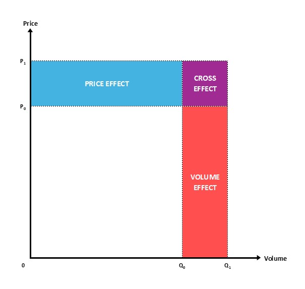
- Price Effect = (P₁ – P₀) × Q₀ “What would we have gained/lost if only prices had changed?”
- Volume Effect = (Q₁ – Q₀) × P₀ “What would we have gained/lost if only volumes had changed?”
- Cross Effect = (P₁ – P₀) × (Q₁ – Q₀) “The interaction between price and volume changes”
Practical Example
Period 0: 1,000 units at $50 = $50,000
Period 1: 1,100 units at $52 = $57,200
Total Change = $7,200
Breaking it down:
- Price Effect = ($52 – $50) × 1,000 = $2,000
- Volume Effect = (1,100 – 1,000) × $50 = $5,000
- Cross Effect = ($52 – $50) × (1,100 – 1,000) = $200
Verification: $2,000 + $5,000 + $200 = $7,200 ✓
Interpretation: The revenue growth was primarily driven by volume (+70%), with price increases contributing 28%, and 2% from their interaction.
Multi-Product Analysis: Introducing Mix Effect
When analyzing a portfolio of products with different prices, the mix effect becomes crucial. It measures the impact of changes in the sales composition.
Why Mix Matters
Consider a company selling:
- Premium products at $100 (high margin)
- Standard products at $50 (medium margin)
- Entry products at $25 (low margin)
Even if total volume remains constant, shifting sales toward premium products increases revenue (positive mix effect), while shifting toward entry products decreases it (negative mix effect).
The Three-Effect Decomposition Method
For multi-product analysis, the most rigorous approach decomposes revenue change into three pure effects:
1. Pure Price Effect
Formula: Σ(Price₁ – Price₀) × Volume₁
Measures: The impact of price changes applied to actual Period 1 volumes.
Example:
- Premium: ($160 – $150) × 180 = +$1,800
- Standard: ($85 – $80) × 550 = +$2,750
- Entry: ($35 – $40) × 900 = -$4,500
- Price Effect = $50
Interpretation: Price increases on premium and standard products were almost entirely offset by a price reduction on the entry product.
2. Pure Volume Effect
Formula: (Total Volume₁ – Total Volume₀) × Average Price₀
Measures: The impact of total volume change, assuming both mix and prices remain constant.
Example:
- Total Volume₀ = 1,500 units
- Total Volume₁ = 1,630 units
- Average Price₀ = $68
- Volume Effect = (1,630 – 1,500) × $68 = $8,840
3. Mix Effect
Formula: Σ(Price₀ × Volume₁) – (Total Volume₁ × Average Price₀)
Measures: The impact of composition change at constant prices.
Calculation Steps:
- Calculate theoretical revenue with Period 1 volumes at Period 0 prices for each product
- Calculate theoretical revenue if mix had remained constant (Total Volume₁ × Average Price₀)
- The difference is the mix effect
Example:
- Theoretical revenue (P₀ prices, P₁ volumes) = $107,000
- Theoretical revenue (constant mix) = 1,630 × $68 = $110,840
- Mix Effect = $107,000 – $110,840 = -$3,840
Interpretation: The company sold relatively more low-priced products and fewer high-priced products, creating a negative mix effect.
Complete Example
Company Data
| Product | P₀ | Q₀ | Revenue₀ | P₁ | Q₁ | Revenue₁ |
|---|---|---|---|---|---|---|
| Premium | $150 | 200 | $30,000 | $160 | 180 | $28,800 |
| Standard | $80 | 500 | $40,000 | $85 | 550 | $46,750 |
| Entry | $40 | 800 | $32,000 | $35 | 900 | $31,500 |
| TOTAL | $68 | 1,500 | $102,000 | $65.7 | 1,630 | $107,050 |
Revenue Change = $5,050
Analysis:
- Price Effect: +$50 (price changes nearly neutral)
- Volume Effect: +$8,840 (58% growth in volume)
- Mix Effect: -$3,840 (shift toward lower-priced products)
Verification: $8,840 – $3,840 + $50 = $5,050 ✓
Understanding the Mix Shift
Volume Share Analysis:
| Product | Share₀ | Share₁ | Change |
|---|---|---|---|
| Premium | 13.3% | 11.0% | -2.3 pts |
| Standard | 33.3% | 33.7% | +0.4 pts |
| Entry | 53.3% | 55.2% | +1.9 pts |
The premium product lost market share while the entry product gained, explaining the negative mix effect despite overall volume growth.
Excel Calculation File
The Cross Effect vs. Mix Effect: Understanding the Difference
Students often confuse these two concepts. Here’s the distinction:
Cross Effect
- Appears in: Single-product analysis
- Nature: Mathematical artifact from sequential decomposition
- Formula: (ΔPrice) × (ΔVolume)
- Business meaning: Limited – it’s the interaction between price and volume changes
- Example: If you raise price by $2 and sell 100 more units, the cross effect is $2 × 100 = $200
Mix Effect
- Appears in: Multi-product analysis only
- Nature: Strategic business indicator
- Formula: Σ(P₀ × Q₁) – (ΣQ₁ × Average Price₀)
- Business meaning: Critical – shows if you’re moving up-market or down-market
- Cannot exist: With only one product
Key Insight: In multi-product analysis, both can coexist but measure completely different phenomena.
Methodological Considerations
Choosing the Right Method
There are two main approaches for multi-product analysis:
Method 1: Sequential by Product (4 effects)
- Calculate Price, Volume, and Cross effects for each product
- Sum them up
- Does NOT explicitly isolate mix effect
- Mix effect is implicit in the volume effects
Method 2: Global Three-Effect Decomposition (Recommended)
- Pure Price Effect (price changes)
- Pure Volume Effect (total volume change)
- Pure Mix Effect (composition change)
- No cross effect residual
- Advantage: Clean separation, exact decomposition, no ambiguity
Common Pitfalls
- Mixing Methods: Using Method 1 for products but trying to add a separate mix calculation creates double-counting or gaps.
- Reference Period Choice: Results depend on which period you use as reference. Be consistent.
- Averaging Errors: Don’t average prices in the “TOTAL” row of tables – this is meaningless. Only volumes and revenues should be summed.
- Attribution Ambiguity: The sequential method attributes the cross effect differently depending on calculation order.
Practical Applications
Strategic Decision-Making
Scenario Analysis Using PVM:
If your analysis shows:
- Positive Volume, Positive Price, Negative Mix: You’re growing but trading down. Consider: Are you sacrificing brand positioning for volume?
- Negative Volume, Positive Price, Positive Mix: You’re losing volume but improving quality/margins. Consider: Is this a deliberate premiumization strategy?
- Positive Volume, Negative Price, Positive Mix: You’re gaining share in premium segments despite competitive pricing. Consider: Can you restore pricing power?
Performance Evaluation
PVM analysis helps evaluate different business units fairly:
| Business Unit | Revenue Change | Volume | Price | Mix | Assessment |
|---|---|---|---|---|---|
| Unit A | +15% | +10% | -3% | +8% | Strong growth, trading up, but pricing pressure |
| Unit B | +5% | +12% | +2% | -9% | Growing volume but losing premium customers |
| Unit C | -5% | -2% | -4% | +1% | Declining market, pricing collapse despite better mix |
Communication to Stakeholders
PVM provides a compelling narrative for explaining performance:
“While our revenue increased by 5%, this modest growth masks significant underlying dynamics. We successfully grew volumes by 9%, and our pricing held firm with a 0.1% increase. However, we experienced a 4% negative mix effect as customers shifted toward value products due to economic conditions. Our strategy for next quarter focuses on rebalancing the portfolio…”
Advanced Topics
Handling Product Launches and Discontinuations
When products didn’t exist in Period 0:
- Exclude from mix calculation
- Report separately as “new product contribution”
- Adjust total volume baseline accordingly
Currency Effects
For international businesses:
- Add a fourth effect: Foreign Exchange
- Perform PVM in constant currency first
- Apply FX effect to constant-currency revenue
Seasonal Businesses
- Compare like periods (Q1 vs Q1, not Q1 vs Q4)
- Use rolling 12-month averages
- Seasonality can create artificial mix effects
Conclusion
Price-Volume-Mix analysis transforms a simple revenue variance into actionable business intelligence. By understanding whether growth comes from volume expansion, price improvements, or portfolio upgrading, managers can:
- Allocate resources more effectively
- Set realistic targets based on controllable levers
- Identify risks such as unfavorable mix shifts
- Communicate performance with clarity and credibility
The key to mastering PVM analysis is:
- Choosing the right methodology for your product portfolio
- Being consistent in application over time
- Connecting the numbers to strategy rather than just reporting them
- Understanding the business context behind each effect
Remember: PVM analysis doesn’t tell you what to do – it tells you what happened and helps you ask the right questions about what to do next.
Leave a Reply